Plotting simulations & residuals spectra#
Simulations and data as well as covariance are stored as sacc objects. For more details regarding sacc format, you can have a look to the tutorial notebooks or you can refer to the official documentation. Here we will read the power spectra for all the simulations and compare its mean value to theory + foregrounds (without and with systematics). As we will see, the content of each spectrum (multipole range, spectra, associated covariance…) is stored within the spec_meta attribute of MFLike. In this tutorial, we will see how to dig into this attribute to plot simulated data against models.
We first start by using the likelihood declaration from the first tutorial
%run tutorial_loading.ipynb
As we did in the foreground tutorial, we first get the theory spectra
model.logposterior({})
dls = model.theory["camb"].get_Cl(ell_factor=True)
To take into account the systematics, we call the mflike.get_modified_theory function. In this function, we need to use the same \(\ell\) range set by the data through the variable l_bpws, that is why we generated the theory spectra using the mflike.l_bpws ell range. (Notice that dls has a multipole range of 2, mflike.l_bpws[-1]).
ell = mflike.l_bpws
dls_cmb = {mode: dls[mode][ell] for mode in ["tt", "te", "ee", "bb"]}
foreground_model = model.theory["mflike.BandpowerForeground"]
fg_totals = foreground_model.get_fg_totals()
dl_obs = mflike.get_modified_theory(dls_cmb, fg_totals, **nuisance_params)
There would be a difference between theory, foreground and the total spectra modified by the systematics once some of the nuisance_parameters are set to a non-ideal value.
Simulated data vs. data model#
We start by plotting unbinned theory + foreground model with the total power spectrum modified by the systematics for a bunch of simulated files. Let’s first start by retrieving the foreground model as a dictionary
fg_models = foreground_model.get_foreground_model(ell=ell, **fg_params)
To load MFLike for different simulated data file, we will use the external way as described in the last part of this tutorial. Altough the spec_meta attribute holds the different spectra, there is no easy way to extract a specific cross and/or mode. Here we will built a dictionary indexed on spectrum mode and cross experiments to be latter used by the plotting function (the contextmanager is just to catch and flush the logging messages when initializing MFLike likelihood)
import logging
from contextlib import contextmanager

from tqdm.auto import tqdm

from mflike import TTTEEE


@contextmanager
def disable_logging(highest_level=logging.CRITICAL):
    previous_level = logging.root.manager.disable
    logging.disable(highest_level)
    try:
        yield
    finally:
        logging.disable(previous_level)


nsims = 10
dls_sims = {}
for isim in tqdm(range(nsims)):
    input_file = dict(input_file=f"LAT_simu_sacc_{isim:05d}.fits")
    with disable_logging():
        ext_mflike = TTTEEE(mflike_input_file | input_file, packages_path=packages_path)
        for data in ext_mflike.spec_meta:
            lb, db = data.get("leff"), data.get("cl_data")
            cross = (data.get("t1"), data.get("t2"))
            mode = data.get("pol") if not data.get("hasYX_xsp") else "et"
            dls_sims.setdefault((mode, *cross), []).append([lb, db])
Warning: The FITS format without the 'sacc_ordering' column is deprecated
Assuming data rows are in the correct order as it was before version 1.0.
Warning: The FITS format without the 'sacc_ordering' column is deprecated
Assuming data rows are in the correct order as it was before version 1.0.
Warning: The FITS format without the 'sacc_ordering' column is deprecated
Assuming data rows are in the correct order as it was before version 1.0.
Warning: The FITS format without the 'sacc_ordering' column is deprecated
Assuming data rows are in the correct order as it was before version 1.0.
Warning: The FITS format without the 'sacc_ordering' column is deprecated
Assuming data rows are in the correct order as it was before version 1.0.
Warning: The FITS format without the 'sacc_ordering' column is deprecated
Assuming data rows are in the correct order as it was before version 1.0.
Warning: The FITS format without the 'sacc_ordering' column is deprecated
Assuming data rows are in the correct order as it was before version 1.0.
Warning: The FITS format without the 'sacc_ordering' column is deprecated
Assuming data rows are in the correct order as it was before version 1.0.
Warning: The FITS format without the 'sacc_ordering' column is deprecated
Assuming data rows are in the correct order as it was before version 1.0.
Warning: The FITS format without the 'sacc_ordering' column is deprecated
Assuming data rows are in the correct order as it was before version 1.0.
Warning: The FITS format without the 'sacc_ordering' column is deprecated
Assuming data rows are in the correct order as it was before version 1.0.
Warning: The FITS format without the 'sacc_ordering' column is deprecated
Assuming data rows are in the correct order as it was before version 1.0.
Warning: The FITS format without the 'sacc_ordering' column is deprecated
Assuming data rows are in the correct order as it was before version 1.0.
Warning: The FITS format without the 'sacc_ordering' column is deprecated
Assuming data rows are in the correct order as it was before version 1.0.
Warning: The FITS format without the 'sacc_ordering' column is deprecated
Assuming data rows are in the correct order as it was before version 1.0.
Warning: The FITS format without the 'sacc_ordering' column is deprecated
Assuming data rows are in the correct order as it was before version 1.0.
Warning: The FITS format without the 'sacc_ordering' column is deprecated
Assuming data rows are in the correct order as it was before version 1.0.
Warning: The FITS format without the 'sacc_ordering' column is deprecated
Assuming data rows are in the correct order as it was before version 1.0.
Warning: The FITS format without the 'sacc_ordering' column is deprecated
Assuming data rows are in the correct order as it was before version 1.0.
Warning: The FITS format without the 'sacc_ordering' column is deprecated
Assuming data rows are in the correct order as it was before version 1.0.
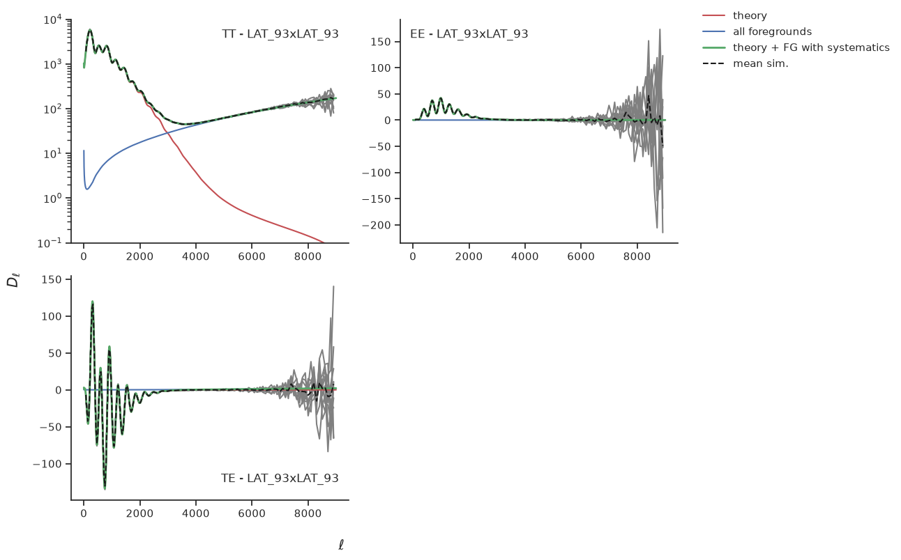
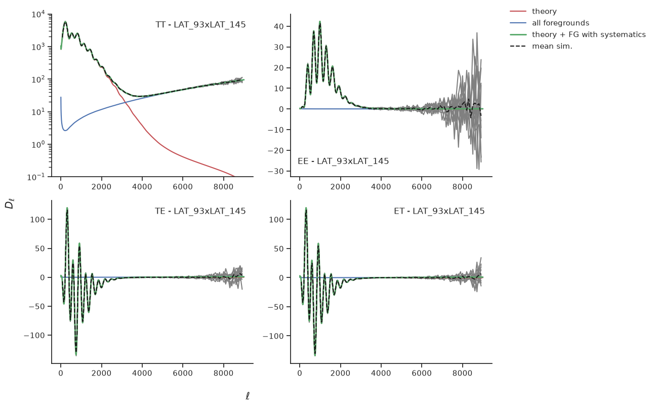
Finally, we can plot the different simulated spectra on top of the CMB expectation + the foreground model
import matplotlib.pyplot as plt


def plot_simulation(*cross):
    fig, axes = plt.subplots(2, 2, figsize=(10, 8))
    for mode, ax in zip(["tt", "ee", "te", "et"], axes.flatten()):
        if not (dls_sim := dls_sims.get((mode, *cross))):
            fig.delaxes(ax)
            continue
        ax.legend([], title="{} - {}x{}".format(mode.upper(), *cross))
        if mode == "tt":
            ax.set(yscale="log", ylim=(0.1, 10_000))

        mode = "te" if mode == "et" else mode
        for lb, db in dls_sim:
            ax.plot(lb, db, "gray")
        ax.plot(ell, dls_cmb[mode], "-r", label="theory")
        ax.plot(ell, fg_models[mode, "all", *cross], "-b", label="all foregrounds")
        ax.plot(ell, dl_obs[mode, *cross], "-g", lw=2, label="theory + FG with systematics")
        ax.plot(*np.mean(dls_sim, axis=0), "--k", label="mean sim.")

    fig.supxlabel(r"$\ell$")
    fig.supylabel(r"$D_\ell$")
    fig.legend(*axes[0, 0].get_legend_handles_labels(), bbox_to_anchor=(1.3, 1))
plot_simulation("LAT_93", "LAT_93")
plot_simulation("LAT_93", "LAT_145")
Plotting residuals#
Given a simulation file, we will loop over the content of MFLike.spec_meta attribute to plot the residuals i.e. simulations - (theory + foregrounds with possible systematics) for the different spectra and cross frequencies. The bandpower weights are stored within the bpw field of spec_meta and we use it to bin the theory and foregrounds spectra
from itertools import combinations_with_replacement as cwr

modes = ["tt", "ee", "te", "et"]

experiments = mflike.experiments
crosses = list(cwr(experiments, 2))
fig, axes = plt.subplots(len(crosses), 4, sharex=True, figsize=(16, 2 * len(crosses)))

for data in mflike.spec_meta:
    # Data/simulation
    lb = data.get("leff")
    db = data.get("cl_data")
    ids = data.get("ids")
    cov = mflike.cov[np.ix_(ids, ids)]
    db_err = np.sqrt(np.diag(cov))

    # Fit
    cross = (data.get("t1"), data.get("t2"))
    db_fit = dl_obs[data.get("pol"), *cross] @ data["bpw"].weight
    delta_db = db - db_fit

    irow = crosses.index(cross)
    mode = data.get("pol") if not data.get("hasYX_xsp") else "et"
    icol = modes.index(mode)
    ax = axes[irow, icol]
    if mode == "tt":
        ax.errorbar(lb, lb**2 * delta_db, lb**2 * db_err, fmt=f".C{icol}")
    else:
        ax.errorbar(lb, delta_db, db_err, fmt=f".C{icol}")

    chi2 = delta_db @ np.linalg.inv(cov) @ delta_db
    title = "{} - {}x{}\n$\chi2$/ndf = {:.2f}".format(mode.upper(), *cross, chi2 / len(delta_db))
    ax.legend([], title=title)

# Remove empty axes
for ax in axes.flatten():
    if not ax.lines:
        fig.delaxes(ax)
for ax in axes[:, 0]:
    ax.set_ylabel(r"$\ell^2\Delta D_\ell$")
for ax in axes[:, 1:].flatten():
    ax.set_ylabel(r"$\Delta D_\ell$")
for ax in axes[-1]:
    ax.set_xlabel(r"$\ell$")
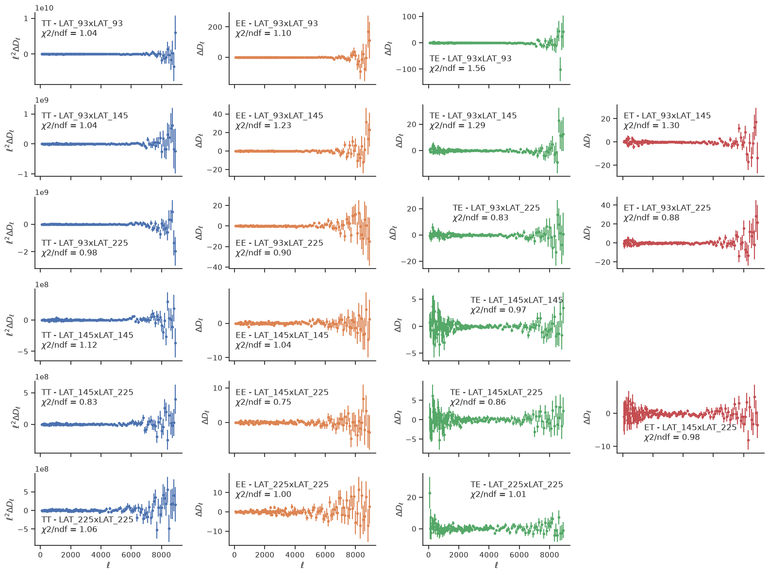
Notice that here the difference between simulations and the (theory+foreground) spectra with possible systematics is mainly driven by the different foreground model adopted by the code