Computing likelihood value#
Given a successful installation of MFLike data (see tutorial), we can now retrieve likelihood or \(\chi^2\) value given the set of parameter values. First, let’s load the MFLike instance
%run tutorial_loading.ipynb
We can retrieve informations related to likelihood(s) as follow
loglikes, derived = model.loglikes()
print(f"log-likelihood value = {loglikes}")
log-likelihood value = [-3585.60572375]
We can directly catch the value returned by logp function from MFLike likelihood
logp = mflike.logp(**fg_params, **nuisance_params)
print(f"log-likelihood value = {logp}")
print(f"Χ² value = {-2 * (logp - mflike.logp_const)}")
log-likelihood value = -3585.6057237523464
Χ² value = 3094.847242785413
Finally, we can also use the evaluate sampler that evaluates the log-likelihood at a given reference point
from cobaya.run import run

info["sampler"] = {"evaluate": None}
updated_info, products = run(info)
[camb] `camb` module loaded successfully from /home/docs/checkouts/readthedocs.org/user_builds/lat-mflike/envs/latest/lib/python3.11/site-packages/camb
Warning: The FITS format without the 'sacc_ordering' column is deprecated
Assuming data rows are in the correct order as it was before version 1.0.
Warning: The FITS format without the 'sacc_ordering' column is deprecated
Assuming data rows are in the correct order as it was before version 1.0.
[mflike.ttteee] Number of bins used: 3087
[mflike.ttteee] Initialized!
[evaluate] *WARNING* No sampled parameters requested! This will fail for non-mock samplers.
[evaluate] Initialized!
[evaluate] Looking for a reference point with non-zero prior.
[evaluate] Reference point:
[evaluate] Evaluating prior and likelihoods...
[evaluate] log-posterior  = -3585.61
[evaluate] log-prior      = 0
[evaluate]    logprior_0 = 0
[evaluate] log-likelihood = -3585.61
[evaluate]    chi2_mflike.TTTEEE = 7171.21
[evaluate] Derived params:
Using the MFLike likelihood without cobaya#
The MFLike likelihood can also be used independently of cobaya. The principle is the same as in
this cobaya’s example. First we need
to instantiate an MFLike object
from mflike import TTTEEE, BandpowerForeground

ext_mflike = TTTEEE(mflike_input_file, packages_path=packages_path)
foreground_model = BandpowerForeground(ext_mflike.get_fg_requirements())
Warning: The FITS format without the 'sacc_ordering' column is deprecated
Assuming data rows are in the correct order as it was before version 1.0.
Warning: The FITS format without the 'sacc_ordering' column is deprecated
Assuming data rows are in the correct order as it was before version 1.0.
[mflike.ttteee] Number of bins used: 3087
[mflike.ttteee] Initialized!
The \(C_\ell\) dictionary can be retrieved from an independant program or an independant computation. Here we will use CAMB to compute the \(C_\ell\) from a cosmological model set by the cosmo_params
camb_cosmo = cosmo_params | minimal_settings
camb_cosmo.update(lmax=ext_mflike.lmax_theory + 1)

pars = camb.set_params(**camb_cosmo)
results = camb.get_results(pars)
powers = results.get_cmb_power_spectra(pars, CMB_unit="muK")
dls_camb = {k: powers["total"][:, v] for k, v in {"tt": 0, "ee": 1, "te": 3, "bb": 2}.items()}
We also get the \(D_\ell\) from cobaya (see tutorial)
dls_cobaya = model.theory["camb"].get_Cl(ell_factor=True)
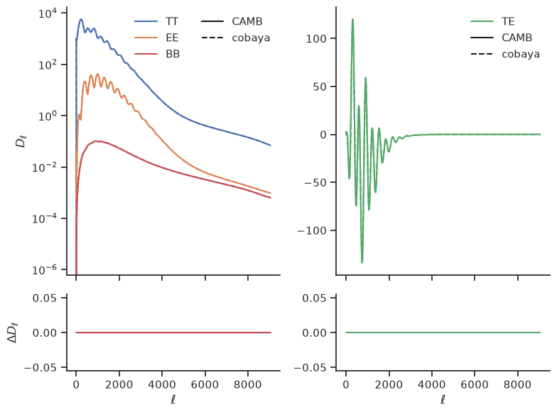
Let’s plot \(D_\ell\) and let’s compare them to the ones from cobaya
import matplotlib.pyplot as plt

fig = plt.figure(figsize=(8, 6))
gs = fig.add_gridspec(4, 2)
axes = {
    "tt": [fig.add_subplot(gs[:3, 0], xticklabels=[]), fig.add_subplot(gs[-1, 0])],
    "te": [fig.add_subplot(gs[:3, 1], xticklabels=[]), fig.add_subplot(gs[-1, 1])],
}


ell = dls_cobaya["ell"]
for i, mode in enumerate(dls_camb):
    plot = axes["te"][0].plot if mode == "te" else axes["tt"][0].semilogy
    plot(ell, dls_camb[mode], f"-C{i}", label=mode.upper())
    plot(ell, dls_cobaya[mode], f"--C{i}")
    ax = axes["te"][1] if mode == "te" else axes["tt"][1]
    ax.plot(ell, dls_camb[mode] - dls_cobaya[mode], f"-C{i}")

axes["tt"][0].set_ylabel(r"$D_\ell$")
axes["tt"][1].set_ylabel(r"$\Delta D_\ell$")
for mode in axes:
    axes[mode][1].set_xlabel(r"$\ell$")
    axes[mode][0].plot([], [], "-k", label="CAMB")
    axes[mode][0].plot([], [], "--k", label="cobaya")
    axes[mode][0].legend(ncol=1 if mode == "te" else 2)
To compute the log-likelihood value, we can use the loglike function which takes as parameters an theoretical \(C_\ell\) dictionary and the nuisance parameter values. We can inject these \(D_\ell\) into the loglike function to get the corresponding log-likelihood value
fg_dict = foreground_model.get_foreground_model_totals(**fg_params)
loglike = ext_mflike.loglike(dls_camb, fg_dict, **nuisance_params)
print(f"log-likelihood value = {loglike}")
print(f"Χ² value = {-2 * (loglike - ext_mflike.logp_const)}")
log-likelihood value = -3585.6057237523464
Χ² value = 3094.847242785413
This way, MFLike likelihood is almost agnostic with respect to the sampler and can be used by others programs than cobaya as far as these programs provide \(D_\ell\) spectra.