Show code cell source

Hide code cell source

import seaborn as sns

sns.set_theme(
    rc={
        "axes.spines.top": False,
        "axes.spines.right": False,
        "figure.autolayout": True,
        "legend.frameon": False,
    },
    style="ticks",
)

Plotting CMB & foreground model

In this tutorial, we will see how to access the foreground model from MFLike and how to plot its components in comparison with the CMB theory spectra. To avoid duplicating code, we load the first tutorial of this serie. This way we have access to the MFLike instance through the variable mflike.

%run tutorial_loading.ipynb

Plotting CMB power spectra

We can get the \(D_\ell\)s from camb using cobaya interface (the call of logposterior method is needed to trigger the \(D_\ell\) computation).

model.logposterior({})
dls_cmb = model.theory["camb"].get_Cl(ell_factor=True)

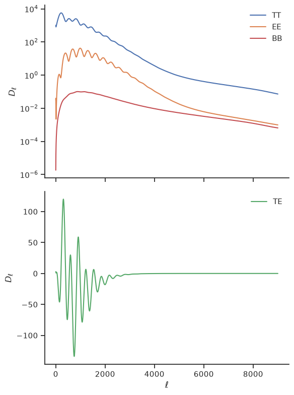
Let’s plot the different spectra on the default multipole range used by MFLike.

import matplotlib.pyplot as plt

ell = mflike.l_bpws

fig, axes = plt.subplots(2, 1, sharex=True, figsize=(6, 8))
for i, mode in enumerate(["tt", "ee", "te", "bb"]):
    ax = axes[1] if mode == "te" else axes[0]
    ax.plot(ell, dls_cmb[mode][ell], f"-C{i}", label=mode.upper())

for ax in axes:
    ax.set_ylabel(r"$D_\ell$")
    ax.legend()
axes[0].set_yscale("log")
axes[1].set_xlabel(r"$\ell$");

Plotting foregrounds

MFLike foreground model can be accessed through the get_foreground_model function of the BandpowerForeground instance. In principle, we can generate a foreground model at higher \(\ell\) than the theory through the ell argument; here we keep the same \(\ell\) range to plot the foregrounds with the theory in the next cell.

foreground_model = model.theory["mflike.BandpowerForeground"]
fg_models = foreground_model.get_foreground_model(ell=ell, **fg_params)

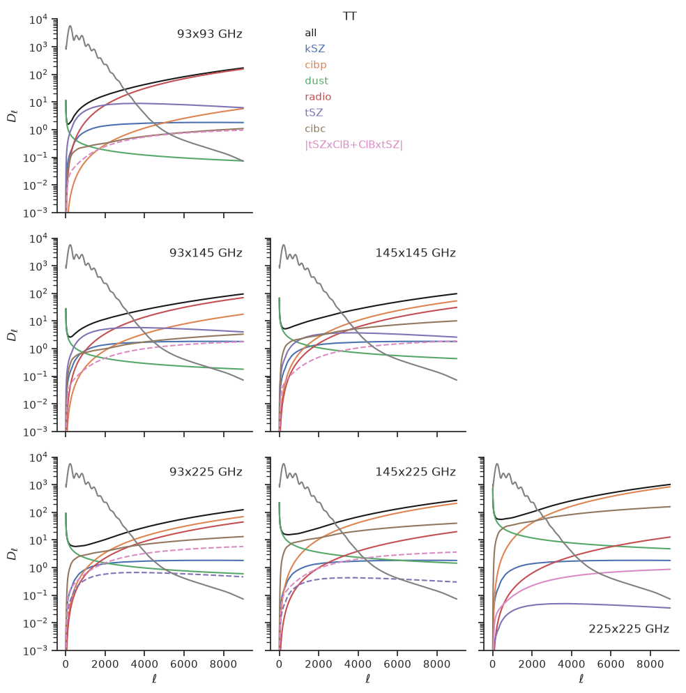
We can then plot theory and foregrounds in a triangle plot given the combinations of cross-frequencies. In the following cell we are just making some adjustments on the foreground components to plot tSZ and cibc autospectrum and their cross correlation separately.

import copy

components = copy.deepcopy(foreground_model.components)
components["tt"].remove("tSZ_and_CIB")
components["tt"] += ["tSZ", "cibc", "tSZxCIB"]

Here we define the plotting function. In the following plots, the dashed lines represent the absolute value of negative spectra.

from itertools import product


def plot_spectra(mode):
    experiments = mflike.experiments
    nexperiments = len(experiments)
    fig, axes = plt.subplots(nexperiments, nexperiments, sharex=True, sharey=True, figsize=(10, 10))

    for i, cross in enumerate(product(experiments, experiments)):
        idx = (i % nexperiments, i // nexperiments)
        ax = axes[idx]
        if idx in zip(*np.triu_indices(nexperiments, k=1)):
            fig.delaxes(ax)
            continue

        ax.plot(ell, fg_models[mode, "all", cross[0], cross[1]], color="k")
        for compo in components[mode]:
            fg_model = fg_models[mode, compo, cross[0], cross[1]]
            if np.any(fg_model < 0):
                ax.plot(ell, np.abs(fg_model), ls="--")
            else:
                ax.plot(ell, fg_model)

        if mode != "te":
            ax.plot(ell, dls_cmb[mode][ell], color="gray")
        else:
            ax.plot(ell, np.abs(dls_cmb[mode][ell]), color="gray", ls="--")
        title = f"{cross[0].split('_')[-1]}x{cross[1].split('_')[-1]} GHz"
        ax.legend([], title=title)
        ax.set(yscale="log", ylim=(0.001, 10_000) if mode == "tt" else None)

    comp_name = copy.deepcopy(components)
    comp_name["tt"] = ["|tSZxCIB+CIBxtSZ|" if n == "tSZxCIB" else n for n in comp_name["tt"]]
    for i in range(nexperiments):
        axes[-1, i].set_xlabel("$\ell$")
        axes[i, 0].set_ylabel("$D_\ell$")
    fig.legend(
        ["all"] + comp_name[mode],
        title=mode.upper(),
        labelcolor="linecolor",
        handlelength=0,
        bbox_to_anchor=(0.6, 1),
    )

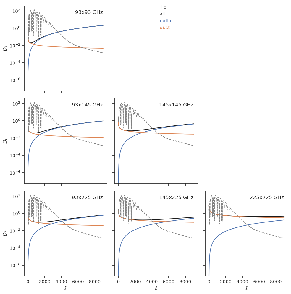
plot_spectra("tt")

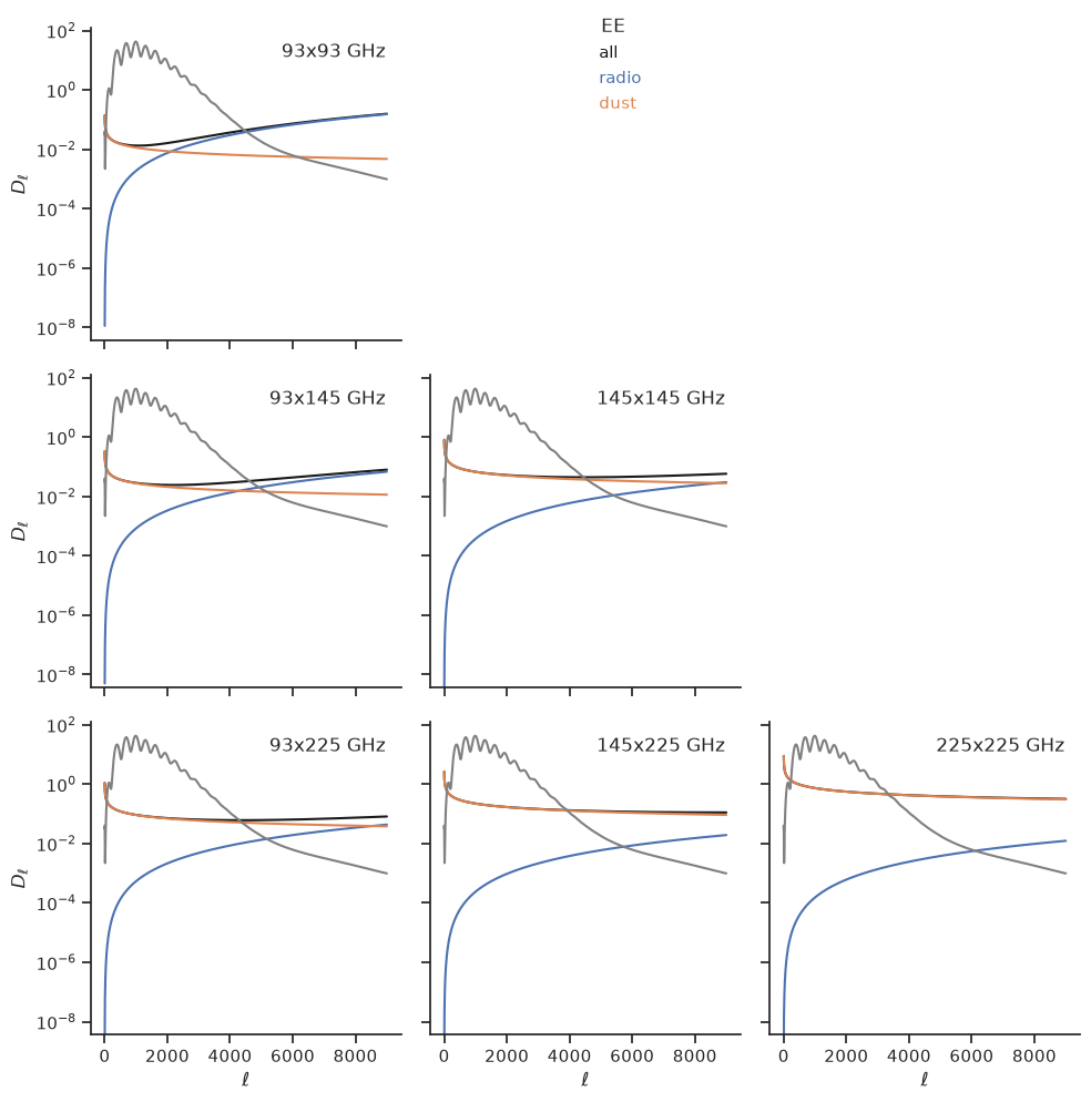
We can also plot the ee or te modes with the argument of the plotting function, to see the contribution from radio and dust components

plot_spectra("ee")

plot_spectra("te")