Show code cell source

Hide code cell source

import seaborn as sns

sns.set_theme(
    rc={"axes.spines.top": False, "axes.spines.right": False, "figure.autolayout": True},
    style="ticks",
)

Fisher matrix

Let’s start by getting the MFLike instance from the first tutorial

%run tutorial_loading.ipynb

Even if we do not need priors to compute Fisher matrix, we need to fool cobaya in order to change parameter values. We set the prior values to ± 10% around the central value (or to a fixed window for parameters whose default is 0).

def fake_priors(value):
    if value == 0:
        min, max = -0.5, +0.5
    else:
        min, max = np.array([0.9, 1.1]) * value
    if value < 0:
        min, max = max, min
    return dict(min=min, max=max)


sampled_params = cosmo_params | fg_params | nuisance_params
sampled_params.update({k: dict(prior=fake_priors(v)) for k, v in sampled_params.items()})

Then we define a new model (after having close the previous one to release memory allocation) and get the MFLike likelihood

We are setting low accuracy parameters for this section, since it would otherwise take much more time

from cobaya.model import get_model

info = {
    "params": sampled_params,
    "likelihood": mflike_config,
    "theory": {"camb": {"extra_args": {"lens_potential_accuracy": 1}},
               "mflike.BandpowerForeground": None},
    "packages_path": packages_path,
}

model = get_model(info)
mflike = model.likelihood["mflike.TTTEEE"]
foreground_model = model.theory["mflike.BandpowerForeground"]

[camb] `camb` module loaded successfully from C:\Work\Dist\git\camb\camb
[mflike.mflike] Number of bins used: 3087
[mflike.mflike] Initialized!

Given the sampled parameters, we now set the defaults value of parameters in the same order as the cobaya’s one

default_values = cosmo_params | fg_params | nuisance_params
defaults = {k: default_values[k] for k in model.parameterization.sampled_params()}

and we define the list of Fisher parameters, removing from the list the parameters we don’t want to perturb (for example, all the nuisance parameters + Alens and some temperature foreground values)

fisher_params = [
    par for par in defaults if par not in ["Alens", "T_d", "T_effd"] + list(nuisance_params)
]

For each parameter, we will compute the associated power spectra by slightly modifying the central value of the parameter (±ε). The power spectra are taken from mflike._get_power_spectra given the nuisance parameters and we also need to recompute (if necessary) the theoritical \(C_\ell\)s. The Fisher algorithm is the following (note that it will take its time, because of the large \(\ell\) range and the high accuracy computation of the spectra)

from tqdm.auto import tqdm

deriv = {k: None for k in fisher_params}

for p in (pbar := tqdm(fisher_params)):
    pbar.set_description(f"Processing '{p}' parameter")

    def _get_power_spectra(epsilon):
        point = defaults.copy()
        point.update({p: point[p] * (1 + epsilon) if point[p] != 0 else point[p] + epsilon})
        model.logposterior(point)
        fg_totals = foreground_model.get_fg_totals()
        cl = model.theory["camb"].get_Cl(ell_factor=True)
        return mflike._get_power_spectra(cl, fg_totals, **point)

    epsilon = 0.01
    ps_minus = _get_power_spectra(-epsilon)
    ps_plus = _get_power_spectra(+epsilon)
    if defaults[p] != 0:
        delta = (ps_plus - ps_minus) / (2 * epsilon * defaults[p])
    else:
        delta = (ps_plus - ps_minus) / (2 * epsilon)
    if np.all(delta == 0):
        print(
            f"WARNING: Sampling a parameter '{p}' that do not have "
            "any effect on power spectra! You should remove it from "
            "cobaya parameter dictionary."
        )
        fisher_params.remove(p)
        continue
    deriv[p] = delta

nparams = len(fisher_params)
fisher_matrix = np.empty((nparams, nparams))
for i1, p1 in enumerate(fisher_params):
    for i2, p2 in enumerate(fisher_params):
        fisher_matrix[i1, i2] = deriv[p1] @ mflike.inv_cov @ deriv[p2]
fisher_cov = np.linalg.inv(fisher_matrix)

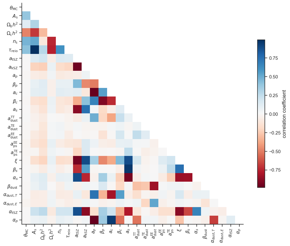
We can show the correlation matrix between parameters

import matplotlib.pyplot as plt

cosmo_labels = dict(
    cosmomc_theta=r"\theta_\mathrm{MC}",
    As=r"A_\mathrm{s}",
    ns=r"n_\mathrm{s}",
    ombh2=r"\Omega_\mathrm{b}h^2",
    omch2=r"\Omega_\mathrm{c}h^2",
    tau=r"\tau_\mathrm{reio}",
)
labels = model.parameterization.labels() | cosmo_labels
latex_names = [rf"${labels[name]}$" for name in fisher_params]

fisher_sigmas = np.sqrt(np.diag(fisher_cov))
norm = np.outer(fisher_sigmas, fisher_sigmas)
fisher_corr = fisher_cov / norm

fig, ax = plt.subplots(figsize=(10, 10))
ind = np.triu_indices_from(fisher_corr)
fisher_corr[ind] = np.nan
im = ax.imshow(fisher_corr, cmap="RdBu")
ax.set_xticks(np.arange(nparams), latex_names, rotation=90)
ax.set_yticks(np.arange(nparams), latex_names, rotation=0)
fig.colorbar(im, shrink=0.5).set_label("correlation coefficient")

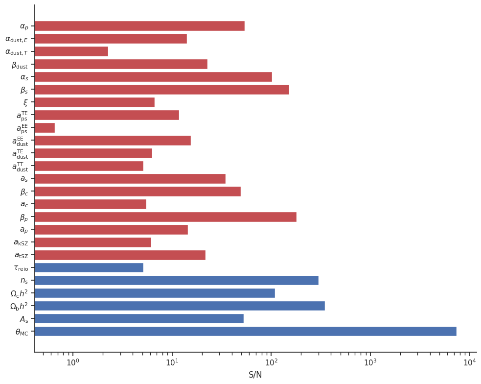
and the Fisher estimated noise

Show code cell source

Hide code cell source

# LaTeX expressions do not render properly with pydata-sphinx-theme.
# It's long standing issue https://github.com/executablebooks/jupyter-book/issues/1826
# with no real solution except hacky's one. Here we convert LaTeX name of parameters to MathML
# equivalent and display the pandas dataframe with the styler class of pandas to render HTML code
# You need to pip install latex2mathml or change index to latex_names variable
# if you do not plan to generate documentation.
import pandas as pd
from latex2mathml.converter import convert

(
    pd.DataFrame(
        [
            [defaults[name], sigma, np.abs(defaults[name] / sigma)]
            for name, sigma in zip(fisher_params, fisher_sigmas)
        ],
        columns=["value", "σ", "Fisher S/N"],
        index=map(convert, [rf"{labels[name]}" for name in fisher_params]),
    )
    .sort_values("Fisher S/N", ascending=False)
    .style.format("{:e}", subset=["value", "σ"])
)

	value	σ	Fisher S/N
${\theta }_{\mathrm{M}\mathrm{C}}$	1.040920e-02	1.405784e-06	7404.553659
${\Omega }_b{h}^2$	2.237000e-02	6.408286e-05	349.079325
$n_s$	9.649000e-01	3.217733e-03	299.869514
${\beta }_p$	2.200000e+00	1.226949e-02	179.306622
${\beta }_s$	-2.500000e+00	1.653964e-02	151.151996
${\Omega }_c{h}^2$	1.200000e-01	1.104581e-03	108.638462
${\alpha }_s$	1.000000e+00	9.758260e-03	102.477290
${\alpha }_p$	1.000000e+00	1.849340e-02	54.073333
$A_s$	2.098903e-09	3.968838e-11	52.884576
${\beta }_c$	2.200000e+00	4.474972e-02	49.162314
$a_s$	3.100000e+00	8.962352e-02	34.589136
${\beta }_{\mathrm{d}\mathrm{u}\mathrm{s}\mathrm{t}}$	1.500000e+00	6.570298e-02	22.830015
$a_{\mathrm{t}\mathrm{S}\mathrm{Z}}$	3.300000e+00	1.515281e-01	21.778140
$a_{\mathrm{d}\mathrm{u}\mathrm{s}\mathrm{t}}^{\mathrm{E}\mathrm{E}}$	1.000000e-01	6.499191e-03	15.386530
$a_p$	6.900000e+00	4.769117e-01	14.468087
${\alpha }_{\mathrm{d}\mathrm{u}\mathrm{s}\mathrm{t},E}$	-4.000000e-01	2.818837e-02	14.190251
$a_{\mathrm{p}\mathrm{s}}^{\mathrm{T}\mathrm{E}}$	4.200000e-02	3.558257e-03	11.803533
$\xi$	1.000000e-01	1.499541e-02	6.668706
$a_{\mathrm{d}\mathrm{u}\mathrm{s}\mathrm{t}}^{\mathrm{T}\mathrm{E}}$	1.000000e-01	1.589361e-02	6.291835
$a_{\mathrm{k}\mathrm{S}\mathrm{Z}}$	1.600000e+00	2.589273e-01	6.179340
$a_c$	4.900000e+00	8.875297e-01	5.520942
$a_{\mathrm{d}\mathrm{u}\mathrm{s}\mathrm{t}}^{\mathrm{T}\mathrm{T}}$	2.800000e+00	5.458397e-01	5.129711
${\tau }_{\mathrm{r}\mathrm{e}\mathrm{i}\mathrm{o}}$	5.440000e-02	1.063018e-02	5.117505
${\alpha }_{\mathrm{d}\mathrm{u}\mathrm{s}\mathrm{t},T}$	-6.000000e-01	2.654750e-01	2.260100
$a_{\mathrm{p}\mathrm{s}}^{\mathrm{E}\mathrm{E}}$	3.000000e-03	4.561110e-03	0.657735

Let’s show the Signal over Noise ratio graphically

fig, ax = plt.subplots(figsize=(10, 8))
signal_over_noise = [np.abs(defaults[name] / sigma) for name, sigma in zip(fisher_params, fisher_sigmas)]
colors = ["b" if name in cosmo_params else "r" for name in fisher_params]
ax.barh(np.arange(nparams), signal_over_noise, color=colors)
ax.set(xscale="log", xlabel="S/N")
ax.set_yticks(range(len(fisher_params)), latex_names);

It also works for TT, TE or EE mode even if you keep the default list of sampled parameters. It will only warn you about the fact that some parameters have no effect on power spectra and thus can be removed from the sampled parameter list.